
Convolution is how a linear, time-invariant system responds to a signal: you flip the system’s impulse response, slide it across the input, and at each step multiply the overlapping samples and add them up. The result, written y[n] = x[n] * h[n], is the system’s output, and it is also exactly how every FIR filter works.
What is convolution, in plain English?
Imagine a echoey room. You clap once, a single sharp pulse, and the room answers with a short burst of echoes that fades away. That echo pattern is the room’s impulse response. Now clap a rhythm instead: every clap produces its own copy of the echo pattern, all overlapping and adding together. The total sound you hear is the sum of all those shifted, overlapping echo copies. That adding-up process is convolution.
Formally, convolution combines an input signal x[n] with a system’s impulse response h[n] to produce the output y[n]. If you know h[n], convolution tells you the output for any input, which is why it sits underneath filtering, echo and reverb, communications channels, and image blurring. If the term impulse response is new to you, read our impulse response lesson first; this lesson uses h[n] throughout.
The method: flip, slide, multiply, sum
Every discrete convolution is the same four steps, repeated for each output sample n:
- Flip h[n] left-to-right, giving h[−k].
- Slide the flipped copy so it sits at position n, giving h[n−k].
- Multiply the overlapping samples of x[k] and h[n−k].
- Sum those products. The total is the single output value y[n].
Move n one step to the right and repeat. That is the whole algorithm, everything else is bookkeeping.
The convolution sum
The four steps above are written as one formula, the convolution sum:
y[n] = Σk=−∞∞ x[k] · h[n−k]
Read it as: “for output sample n, add up every input sample x[k] multiplied by the flipped, shifted impulse response h[n−k].” Two practical facts follow from the formula:
- Output length: if x has length N and h has length M, then y has length N + M − 1.
- Commutativity: x * h = h * x. Sliding x across h gives the same answer, useful as a check on hand calculations.
Worked example: convolve [1, 2, 3] with [0.5, 0.5]
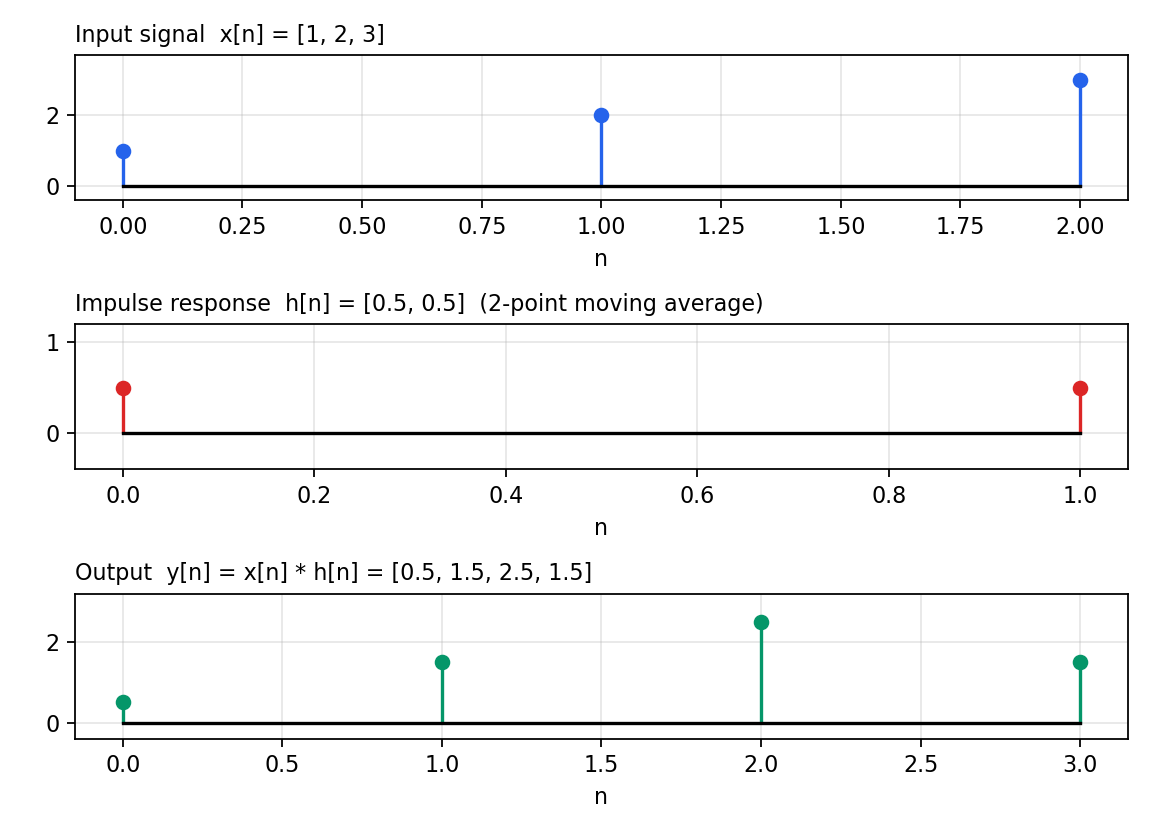
Take x[n] = [1, 2, 3] and h[n] = [0.5, 0.5], a 2-point moving average, the simplest filter there is. The output has length 3 + 2 − 1 = 4. Working through each n:
| Output | Overlapping products | y[n] |
|---|---|---|
| y[0] | 1 × 0.5 | 0.5 |
| y[1] | (1 × 0.5) + (2 × 0.5) | 1.5 |
| y[2] | (2 × 0.5) + (3 × 0.5) | 2.5 |
| y[3] | 3 × 0.5 | 1.5 |
So y[n] = [0.5, 1.5, 2.5, 1.5]. Notice what happened: each interior output is the average of two neighbouring inputs, so the output is a smoothed, slightly longer version of x. That is filtering, done by hand.
Convolution in Python (tested code)
In practice nobody convolves by hand. NumPy does it in one line, and this exact code produced the numbers above:
import numpy as np

x = np.array([1.0, 2.0, 3.0])   # input signal
h = np.array([0.5, 0.5])        # impulse response (2-point average)
y = np.convolve(x, h)           # mode='full' is the default
print(y)                        # [0.5 1.5 2.5 1.5]
To see the flip-slide-multiply-sum method inside that one line, here is the same calculation written out as a loop. Both versions return identical results:
def convolve_manual(x, h):
    y = np.zeros(len(x) + len(h) - 1)
    for n in range(len(y)):          # slide
        for k in range(len(x)):
            if 0 <= n - k < len(h):  # overlap only
                y[n] += x[k] * h[n - k]  # multiply and sum
    return y
For long signals or multi-dimensional data, use scipy.signal.convolve instead, it can switch to an FFT-based method (method='fft'), which computes the same result much faster on large inputs. The mathematics does not change; only the shortcut does.
Why convolution matters: it is how LTI systems work
A system that is linear (outputs add the way inputs add) and time-invariant (it behaves the same today and tomorrow) is completely described by its impulse response h[n]. Feed it any signal, and the output is the convolution of that signal with h[n]. No exceptions, no extra terms.
That single fact is the engine of DSP:
- An FIR filter is a convolution with the filter’s coefficients, the coefficients are h[n].
- A room, a radio channel, a guitar body each convolve your signal with their own impulse response, adding echo and colour.
- Image blur and sharpening are 2-D convolutions with a small kernel, the same operation, one dimension up.
Convolution as smoothing: the moving-average filter
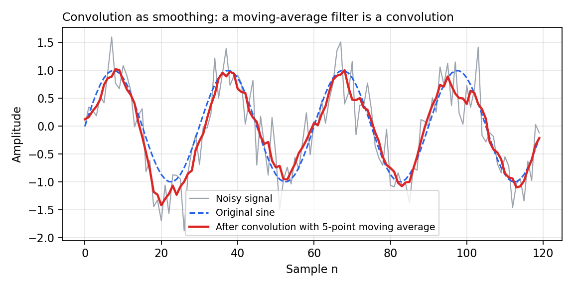
Convolve a noisy signal with h[n] = [0.2, 0.2, 0.2, 0.2, 0.2] and each output sample becomes the average of five neighbouring inputs. Noise jumps up and down sample to sample, so averaging cancels much of it, while the slow underlying signal survives:
This is a real FIR filter, and you can design longer, better ones in your browser: change the coefficients and watch both the impulse response and the frequency response update in our FIR Filter Designer.
Key properties, at a glance
| Property | Rule | Why you care |
|---|---|---|
| Commutative | x * h = h * x | Swap signal and system in a calculation to check your work |
| Associative | (x * h₁) * h₂ = x * (h₁ * h₂) | Two filters in series equal one combined filter |
| Distributive | x * (h₁ + h₂) = x * h₁ + x * h₂ | Parallel filter paths can be analysed separately, then added |
| Output length | N + M − 1 | Explains the “warm-up” samples at the start of filtered audio |
| Frequency view | Convolution in time = multiplication in frequency | The reason FFT-based filtering works at all |
Common mistakes
- Forgetting the flip. Convolution flips h; correlation does not. If your hand result looks like a mirror image of the expected output, you computed a correlation.
- Expecting the output to match the input length. A full convolution returns N + M − 1 samples. Tools that return the input length (NumPy’s
mode='same') are trimming the result. - Blaming the code for edge effects. The first and last M − 1 outputs are computed from partial overlaps, they are correct, but they are transitions, not steady-state filtering.
- Convolving with a non-LTI system. The moment a system clips, quantises coarsely or changes over time, y = x * h stops being the whole story.
Quick quiz
- x has length 10 and h has length 4. How long is the full convolution?
- x = [2, 1], h = [3, 1]. What is y[0]?
- True or false: convolving h * x instead of x * h changes the result.
Answers
- 13 samples (10 + 4 − 1).
- y[0] = 2 × 3 = 6.
- False, convolution is commutative, so the result is identical.
Frequently asked questions
What is the difference between convolution and correlation?
Convolution flips the second sequence before sliding it across the first; correlation slides it without flipping. For symmetric kernels such as a moving average the two give identical results, which is why the difference is often missed. For asymmetric impulse responses the outputs differ, and only convolution describes how an LTI system responds.
Why does convolution flip the signal?
The flip comes from the substitution inside the convolution sum, h[n−k]: as the input index k increases, the impulse-response index n−k decreases, which reverses h. Physically, the earliest input sample has passed through the whole system longest, so it pairs with the last part of the impulse response at each output step.
How long is the output of a convolution?
A full discrete convolution of a length-N signal with a length-M impulse response always has N + M − 1 samples. The extra M − 1 samples are the partial-overlap regions at the start and end, where the flipped impulse response is still sliding into, or out of, the input.
Is convolution the same in images and in audio?
Yes, the operation is identical, extended to two dimensions. An image kernel slides across rows and columns instead of along one time axis, and each output pixel is a weighted sum of its neighbourhood. Blur, sharpening and edge detection filters are all 2-D convolutions with different kernels.
Where to go next
Convolution leans on two ideas you have now met: the impulse response and the idea of a signal as a sequence of samples. Next in the beginner path, see how sampling a signal can go wrong in our aliasing lesson, or step back to what a signal is in DSP. The full order is on the Beginner DSP learning path.
References
- Steven W. Smith, The Scientist and Engineer’s Guide to Digital Signal Processing, Chapter 6, “Convolution”, dspguide.com/ch6.htm
- NumPy documentation: numpy.convolve
- SciPy documentation: scipy.signal.convolve
Try it yourself
Convolution stops being abstract the moment you change a coefficient and watch the output move. Design a windowed-sinc FIR filter, its coefficients are an impulse response, and see its shape and frequency response update live. Open the FIR Filter Designer.
Keep going in order: the Beginner DSP learning path shows what to learn next.