 By DSP Staff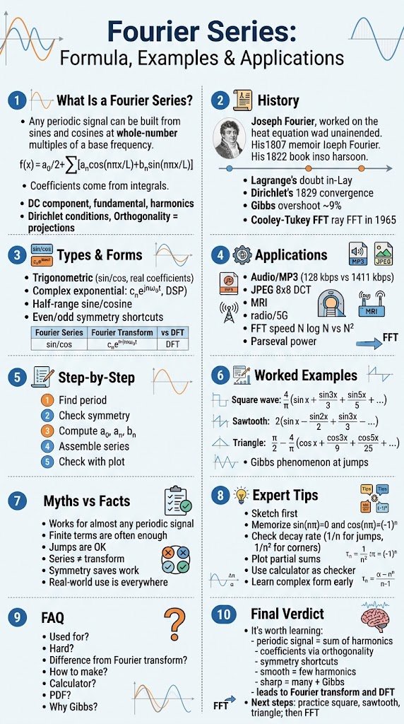
INTRODUCTION
Every sound you have ever heard, from a piano note to your best friend’s voice, is a single wiggling pressure wave. So how does your phone tell a violin from a flute playing the same pitch? The answer starts with a 200-year-old idea: any repeating signal can be built by adding simple sine and cosine waves together. That idea is the Fourier series.
If you study electrical engineering, physics, or signal processing, you will meet the Fourier series in almost every course. It powers MP3 audio, JPEG images, MRI scanners, radio communication, and the heat equation that started it all. Yet many students find it intimidating, because textbooks often jump straight into integrals with no story behind them.
This guide fixes that. You will learn what a Fourier series is in plain language, where it came from, and the different forms it takes. You will see the Fourier series formula, follow a clean derivation, and build a Fourier series expansion step by step with worked examples. You will also learn what it is used for, how it differs from the Fourier transform, and how to check your work with a Fourier series calculator.
By the end, you will not just memorize equations. You will understand why they work, which is what makes exams and real projects feel manageable. Grab a pen, and let’s start with the basics.
TABLE OF CONTENTS
- What Is a Fourier Series?
- Who Invented the Fourier Series? History and Origin
- What Are the Types and Forms of a Fourier Series?
- Why Does the Fourier Series Matter? Benefits and Applications
- How to Make a Fourier Series: Step-by-Step Guide
- Fourier Series Myths vs Facts
- Expert Tips and Best Practices for Learning the Fourier Series
- Frequently Asked Questions
- Final Verdict
What Is a Fourier Series?
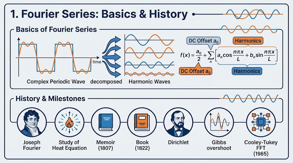
A Fourier series is a way of writing a periodic function as an infinite sum of sines and cosines. Each sine or cosine has a frequency that is a whole-number multiple of one base frequency. Each also carries its own weight, called a Fourier coefficient. Add enough of them, and the sum matches your original function.
Think about mixing paint. With red, yellow, and blue, you can create almost any color. The Fourier series does the same for waves. Sines and cosines are your primary colors, and the coefficients tell you how much of each to pour in.
Here is the standard Fourier series formula for a function f(x) with period 2L:
f(x) = a₀/2 + Σ [ aₙ·cos(nπx/L) + bₙ·sin(nπx/L) ] (sum from n = 1 to ∞)The coefficients come from three integrals, each taken over one full period from −L to L:
a₀ = (1/L) ∫ f(x) dx
aₙ = (1/L) ∫ f(x)·cos(nπx/L) dx
bₙ = (1/L) ∫ f(x)·sin(nπx/L) dx
Let’s decode that. The term a₀/2 is the average value of your signal, which engineers call the DC component. The term with n = 1 is the fundamental frequency, the slowest wave that still fits the period. Terms with n = 2, 3, 4 and so on are the harmonics, waves that vibrate two, three, or four times faster.
Not every function qualifies. A function needs to satisfy the Dirichlet conditions: within one period it must be single-valued, have a finite number of jumps, and have a finite number of peaks and valleys. Nearly every signal you meet in practice passes this test. At a jump, the series settles on the midpoint of the gap.
There is also a deeper view that makes the Fourier series math feel natural. Sines and cosines of different frequencies are orthogonal, which means they do not overlap in a mathematical sense. Think of the x, y, and z axes in 3D space. To find how far a point sits along the x-axis, you project onto it. The Fourier coefficients are exactly those projections, just in a space with infinitely many axes.
This is why the Fourier series is so useful. It turns a complicated shape into a list of numbers, one per frequency. Once you have that list, questions like “how much energy sits at 50 Hz?” become trivial to answer.
Now that you know what a Fourier series is, let’s see how a physics problem about heat gave birth to it.
Who Invented the Fourier Series? History and Origin
The Fourier series carries the name of Joseph Fourier, a French mathematician and physicist born in 1768. But the story begins with a physical puzzle, not a math one: how does heat move through a solid object?
In the early 1800s, Fourier studied heat flow in metal plates and rods. He wrote down the heat equation and noticed something helpful. If the starting temperature looks like a simple sine wave, the solution is easy to find. The trouble is that real temperature patterns are messy.
His bold move was to claim that any starting pattern could be written as a sum of sine waves. Then you solve for each wave separately and add the answers back together. This trick, splitting a hard problem into many easy ones, is still the heart of signal processing today.
Fourier submitted his first major memoir on heat conduction to the Paris Academy of Sciences in December 1807, according to standard historical accounts such as Britannica. The reviewers were not convinced. Joseph-Louis Lagrange, one of the greatest mathematicians of the age, doubted that smooth sine waves could add up to a shape with sharp corners. The memoir was not published at that time. Fourier kept refining his ideas, and his famous book Théorie analytique de la chaleur (The Analytical Theory of Heat) appeared in 1822.
Lagrange had a point, and mathematicians spent the next century sorting it out. Peter Gustav Lejeune Dirichlet gave the first rigorous conditions for convergence in 1829. Bernhard Riemann built parts of his theory of integration to handle Fourier series. Georg Cantor’s early work on when a trigonometric series is unique pushed him toward set theory. In 1966, Lennart Carleson proved a landmark result: the Fourier series of a well-behaved function converges at almost every point.
Along the way, people discovered odd behavior near jumps. The overshoot that appears there is called the Gibbs phenomenon. Henry Wilbraham described it in 1848, and J. Willard Gibbs rediscovered it around 1899. You will see it in action later in this guide.
The last big chapter is computing. In 1965, James Cooley and John Tukey published the Fast Fourier Transform (FFT) algorithm, which made frequency analysis practical on computers. Historians later found that Carl Friedrich Gauss had used a similar trick around 1805, but he never published it in a widely read form. Today the FFT runs inside your phone, your car, and your Wi-Fi router.
With the history in place, let’s look at the different shapes a Fourier series can take.
What Are the Types and Forms of a Fourier Series?
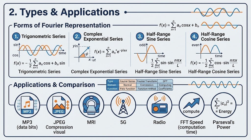
When people search for Fourier series expansion, they usually mean one of several closely related forms. All of them describe the same idea, but each one suits a different situation. Picking the right form saves you a lot of work.
The Trigonometric Form
This is the form you saw earlier, with sines and cosines and real coefficients. It is the most common version in math and physics courses. It works best when you want to see the shape of the signal and do the integrals by hand.
The Complex Exponential Form
Engineers love this version because it has one formula instead of three. Using Euler’s identity, e^(jθ) = cos θ + j·sin θ, you can pack the sine and cosine terms together:
f(t) = Σ cₙ · e^(j·n·ω₀·t)      (sum from n = −∞ to ∞)
cₙ = (1/T) ∫ f(t) · e^(−j·n·ω₀·t) dt
Here T is the period and ω₀ = 2π/T is the fundamental angular frequency. Each coefficient cₙ is a complex number. Its magnitude tells you how strong that frequency is, and its angle tells you the phase, or timing offset. This is the form you will use most in DSP, because it leads directly to the Fourier transform and the DFT.
Half-Range Sine and Cosine Series
Sometimes a function is defined only on a short interval, say from 0 to L, such as the shape of a plucked guitar string. You can extend it to a full period in two ways. An odd extension gives a series with only sine terms. An even extension gives a series with only cosine terms. These half-range series are common in heat and wave problems with fixed boundary conditions.
Shortcuts From Even and Odd Symmetry
Symmetry can cut your work in half. If f(x) is even (a mirror image around the y-axis), all bₙ terms are zero. If f(x) is odd (rotationally symmetric about the origin), all aₙ terms and a₀ are zero. Always check for symmetry before you start integrating.
| Form | Uses | Best for | Coefficients |
|---|---|---|---|
| Trigonometric | sin and cos | Hand calculation, waveform shape | Real (a₀, aₙ, bₙ) |
| Complex exponential | e^(jnω₀t) | DSP, circuits, theory | Complex (cₙ) |
| Half-range sine | sin only | Fixed-end strings, heat problems | Real (bₙ) |
| Half-range cosine | cos only | Insulated-end heat problems | Real (a₀, aₙ) |
Fourier Series vs Fourier Transform vs DFT
Students often mix these three tools. The table below keeps them straight.
| Feature | Fourier Series | Fourier Transform | Discrete Fourier Transform (DFT) |
|---|---|---|---|
| Input signal | Periodic, continuous time | Non-periodic, continuous time | Finite list of samples |
| Output | Discrete set of harmonics | Continuous spectrum | Finite list of frequency values |
| Frequencies | Multiples of a base frequency | Every frequency | N evenly spaced frequencies |
| Typical use | Repeating waves, circuits | Pulses, filters, analysis | Computers, FFT, real data |
The short version: the Fourier series handles repeating signals, the transform handles one-time signals, and the DFT handles data stored in a computer.
Now that you know the forms, let’s talk about why you should care.
Why Does the Fourier Series Matter? Benefits and Applications
The Fourier series applications list is long, because frequency is one of the most useful ways to look at the world. Here are the biggest reasons the tool matters and where you will meet it.
It Turns Hard Problems Into Easy Ones
Solving a differential equation with a messy input is painful. But if you split the input into sine waves, each piece has a simple answer, and you add the answers back together. This works because linear systems treat each frequency independently. It is the reason circuit analysis and vibration analysis rely on Fourier methods.
Audio and Music
Every musical instrument has a unique blend of harmonics, and this blend is called timbre. A clarinet has strong odd harmonics, while a violin has a rich mix of both. Synthesizers build sounds by adding sine waves, which is a Fourier series in action.
Compression also depends on this idea. A standard audio CD stores 44,100 samples per second in 16 bits per channel, which works out to about 1,411 kbps for stereo under the Red Book standard. A typical 128 kbps MP3 is roughly 11 times smaller. MP3 achieves this by moving to the frequency domain and discarding components your ear barely notices.
Images and Video
The JPEG format splits an image into 8×8 blocks and applies a close relative of the Fourier series called the Discrete Cosine Transform, as defined in the ITU-T T.81 standard. Most of the visual information ends up in a few low-frequency coefficients. The tiny high-frequency ones can be thrown away with little visible loss.
Communications and Electronics
Radio, Wi-Fi, and 5G all shape signals in the frequency domain. Engineers use Fourier series to analyze square-wave clocks, power supplies, and distortion in amplifiers. When a square wave passes through a filter and comes out rounded, you can predict exactly what happened by looking at which harmonics were removed.
Medicine and Science
MRI machines collect data in frequency space, then use Fourier methods to reconstruct an image of your body. Astronomers analyze starlight the same way. Chemists use it in infrared spectroscopy. Seismologists use it to study earthquakes.
Speed on Computers
The FFT, a fast method for computing Fourier coefficients, cuts the cost of frequency analysis from roughly N² operations to N·log₂(N). Cooley and Tukey published this algorithm in Mathematics of Computation in 1965. For a signal with one million samples, that is about 50,000 times fewer operations. Without the FFT, real-time audio and video processing would be far too slow.
Energy Insight Through Parseval’s Theorem
Parseval’s theorem says the total power of a signal equals the sum of the power in each harmonic. This gives you a neat way to check your work and to see where a signal’s energy lives.
Each benefit comes from the same idea: look at a signal by frequency, and hard things become simple. Next, you will learn how to make a Fourier series yourself.
How to Make a Fourier Series: Step-by-Step Guide
Let’s get practical. First you will see where the formulas come from, then a repeatable method, then three worked examples.
Fourier Series Derivation in Plain Language
The Fourier series derivation relies on one key fact: sines and cosines are orthogonal over one period. For a period of 2π, these integrals hold for whole numbers m and n (with m, n ≥ 1):
∫ sin(mx)·sin(nx) dx = π   if m = n,  and 0 if m ≠ n
∫ cos(mx)·cos(nx) dx = π   if m = n,  and 0 if m ≠ n
∫ sin(mx)·cos(nx) dx = 0   always
(All integrals run from −π to π.) Now start with the assumed series:
f(x) = a₀/2 + Σ [ aₙ·cos(nx) + bₙ·sin(nx) ]Multiply both sides by cos(mx) and integrate over one period. Because of orthogonality, every term on the right vanishes except the one with n = m. That surviving term equals aₘ·π. Divide by π, and you get aₘ = (1/π) ∫ f(x)·cos(mx) dx. Repeat with sin(mx) to get bₘ. Integrating the original series directly, with no multiplier, gives a₀.
That is the whole trick: multiplying by a sine or cosine “selects” one coefficient and kills the rest.
The Step-by-Step Method
Follow these steps for any function:
- Confirm the function is periodic and find the period. Write down T = 2L. If the function is given only on an interval, decide whether to repeat it (a full-range series) or extend it as even or odd (a half-range series).
- Check for symmetry. If f(x) is even, skip bₙ. If f(x) is odd, skip a₀ and aₙ. This step alone can save you half the work.
- Compute a₀. Integrate f(x) over one period and divide by L. This gives you twice the average value, so your series starts with a₀/2.
- Compute aₙ. Multiply f(x) by cos(nπx/L), integrate over one period, and divide by L. Simplify using the fact that sin(nπ) = 0 and cos(nπ) = (−1)ⁿ for whole numbers n.
- Compute bₙ. Multiply f(x) by sin(nπx/L), integrate, and divide by L. Use the same simplifications.
- Assemble the series. Substitute your coefficients into the main formula. Write out the first three or four nonzero terms so the pattern is visible.
- Check your answer. Plug in a point where you know the answer, or plot a few partial sums and see if they approach the original shape.
Worked Example 1: The Square Wave
Take f(x) = −1 for −π < x < 0 and f(x) = +1 for 0 < x < π, repeating every 2π. This is an odd function, so a₀ = 0 and all aₙ = 0. You only need bₙ:
bₙ = (1/π) ∫ f(x)·sin(nx) dx      (from −π to π)
   = (2/π) ∫ sin(nx) dx           (from 0 to π, because the integrand is even)
   = (2/π) · [ −cos(nx)/n ]       (evaluated from 0 to π)
   = (2/(nπ)) · (1 − cos(nπ))
If n is even, cos(nπ) = 1, so bₙ = 0. If n is odd, cos(nπ) = −1, so bₙ = 4/(nπ). The result is:
f(x) = (4/π) · [ sin(x) + sin(3x)/3 + sin(5x)/5 + sin(7x)/7 + ... ]Now test it. At x = π/2, every sine is ±1, and the series becomes (4/π)(1 − 1/3 + 1/5 − 1/7 + …). That inner sum equals π/4, so the total is exactly 1, which matches f(π/2). A neat bonus: you just proved the Leibniz formula for π.
Worked Example 2: The Sawtooth Wave
Take f(x) = x on (−π, π), repeating every 2π. It is odd, so only bₙ survives. Integration by parts gives bₙ = 2·(−1)ⁿ⁺¹/n, so:
f(x) = 2 · [ sin(x) − sin(2x)/2 + sin(3x)/3 − sin(4x)/4 + ... ]Unlike the square wave, the sawtooth uses every harmonic, and its coefficients shrink slowly, like 1/n. Slow shrinking means sharp jumps.
Worked Example 3: The Triangle Wave
Take f(x) = |x| on (−π, π). It is even, so bₙ = 0. You get a₀ = π, and aₙ = 2((−1)ⁿ − 1)/(πn²), which is −4/(πn²) for odd n and zero for even n:
f(x) = π/2 − (4/π) · [ cos(x) + cos(3x)/9 + cos(5x)/25 + ... ]Notice that these coefficients shrink like 1/n², much faster than the square wave. A smoother signal needs fewer harmonics. This rule of thumb will help you sanity-check your answers.
Seeing the Gibbs Phenomenon
Add more terms to the square-wave series, and the approximation gets better everywhere except right at the jump. There, the partial sums always overshoot by a fixed amount. The overshoot settles at about 9% of the jump height, as described by Wolfram MathWorld, no matter how many terms you add. The overshoot region just gets narrower. This is normal behavior, not a mistake in your calculation.
You now know how to build a Fourier series by hand. Before we go further, let’s clear up some common misunderstandings.
Fourier Series Myths vs Facts
Students pick up a few wrong ideas early, and those ideas cause real confusion on exams. Here are the most common ones.
Myth 1: A Fourier series only works for sine waves.
Fact: It works for almost any periodic signal, including square waves, triangle waves, pulses, and irregular repeating shapes. Sine and cosine are the building blocks, not the target.
Myth 2: You need an infinite number of terms to use it.
Fact: The full series is infinite, but real work uses a partial sum. For many signals, five or ten terms give an excellent match. The smoother the signal, the fewer terms you need.
Myth 3: The series can’t represent functions with jumps.
Fact: It can, and this is exactly what worried Lagrange. The series converges to the function at smooth points and to the midpoint at a jump. The Gibbs overshoot is a side effect, not a failure.
Myth 4: The Fourier series and the Fourier transform are the same thing.
Fact: The series is for periodic signals and produces discrete harmonics. The transform is for non-periodic signals and produces a continuous spectrum. The transform is what you get when the period grows toward infinity.
Myth 5: You must do all three integrals every time.
Fact: Symmetry often makes half of them zero. Even functions need only cosines, and odd functions need only sines.
Myth 6: It’s purely theoretical and has no real use.
Fact: Your phone, your music streaming app, and your doctor’s MRI scanner all depend on Fourier methods every day.
Clearing away these myths sets you up for better learning habits, which is what the next section covers.

Expert Tips and Best Practices for Learning the Fourier Series
After years of teaching and writing about signal processing, I see the same patterns separate students who “get it” from those who struggle. Use these tips to move faster.
1. Look at the picture before the formula. Sketch the function and its periodic extension first. Spotting symmetry or jumps at this stage will save you a page of algebra later.
2. Memorize the shortcut integrals. For whole numbers n, remember that sin(nπ) = 0, cos(nπ) = (−1)ⁿ, and cos(2nπ) = 1. Nearly every textbook problem uses them.
3. Check the coefficients’ decay rate. If your function has jumps, the coefficients should shrink like 1/n. If it is continuous with corners, expect 1/n². If your answer disagrees, look for an algebra slip.
4. Plot partial sums. Nothing builds intuition like watching a square wave emerge from one, three, ten, then fifty sine waves. A short script does the job:
import numpy as np
import matplotlib.pyplot as plt

x = np.linspace(-np.pi, np.pi, 1000)

def square_wave_partial(x, harmonics):
    total = np.zeros_like(x)
    for k in range(harmonics):
        n = 2 * k + 1                      # only odd harmonics
        total += (4 / (np.pi * n)) * np.sin(n * x)
    return total

for h in (1, 3, 10, 50):
    plt.plot(x, square_wave_partial(x, h), label=f"{h} harmonics")

plt.legend()
plt.title("Fourier series of a square wave")
plt.show()
5. Use a Fourier series calculator as a checker, not a crutch. Tools like Wolfram Alpha, Desmos, and Symbolab can compute coefficients and plot partial sums in seconds. Work the problem by hand first, then compare. If the results differ, you have found a learning opportunity.
6. Learn the complex form early. It looks scarier, but it has fewer formulas and leads straight to the Fourier transform and DFT. Most DSP courses assume you are comfortable with it by week four.
7. Connect coefficients to physical meaning. Ask yourself: what does this coefficient represent? Is it the DC level, the fundamental, or the third harmonic? Students who attach meaning to numbers remember them longer.
8. Keep a one-page cheat sheet. Many students search for a Fourier series PDF before exams. Make your own instead, with the main formula, the orthogonality relations, symmetry rules, and three example series. The act of writing it teaches you more than downloading someone else’s.
9. Practice with a fixed set of signals. Master the square, sawtooth, triangle, and rectified sine waves. These four cover a large share of exam questions and real-world signals.
10. Study Parseval’s theorem. It links time-domain power to frequency-domain power and is a great sanity check. For a 2π-periodic signal:
(1/π) ∫ f(x)² dx = a₀²/2 + Σ (aₙ² + bₙ²)11. Move on to the DFT once you’re comfortable. The Fourier series is your foundation. The next step is the Discrete Fourier Transform, where you apply the same ideas to sampled data.
Next, let’s answer the questions students ask most often.
Frequently Asked Questions
What is a Fourier series used for?
A Fourier series is used to break a repeating signal into simple sine and cosine components so you can study each frequency separately. Engineers use it to analyze circuits, design filters, and study distortion in amplifiers. Audio software uses it for equalizers, synthesizers, and MP3 compression. Physicists use it to solve heat, wave, and vibration problems. Imaging systems like JPEG and MRI build on closely related methods. Whenever you need to know “how much of each frequency is in this signal?”, a Fourier series is the tool to reach for.
Is Fourier series hard to learn?
It feels hard at first, but it is more approachable than most students expect. The core idea, building waves from sines and cosines, is simple. The difficulty comes from the integrals and from a pile of new notation. If you are comfortable with basic calculus, trigonometric identities, and integration by parts, you can learn the fundamentals in a few weeks of steady practice. Start with visual examples, master the square and sawtooth waves, and check your results with a plot. The complex form and convergence theory come later and need more patience.
What is the difference between a Fourier series and a Fourier transform?
A Fourier series describes a periodic signal as a sum of harmonics at discrete frequencies: the fundamental, twice the fundamental, three times, and so on. A Fourier transform describes a non-periodic signal using a continuous range of frequencies. You can think of the transform as the series in the limit where the period becomes infinite and the gaps between harmonics shrink to nothing. In practice, you use the series for repeating waves like clocks and AC power, and the transform for one-time events like a single pulse or a spoken word.
How to make a Fourier series?
Start by identifying the period and checking for even or odd symmetry. Then compute a₀, aₙ, and bₙ using the integral formulas over one period. Simplify the results using sin(nπ) = 0 and cos(nπ) = (−1)ⁿ. Finally, plug the coefficients into the series formula and write out the first few terms. Test the result by plugging in a point where you know the answer or by plotting partial sums. The step-by-step section above walks through this process with square, sawtooth, and triangle waves you can copy for practice.
Is there a good Fourier series calculator?
Yes, several. Wolfram Alpha computes coefficients and full series for many functions. Desmos lets you plot partial sums with a slider for the number of terms, which is excellent for building intuition. Symbolab shows step-by-step integration. You can also write a short Python script with NumPy and SciPy, like the one in the tips section. Use calculators to confirm your own work, not replace it, because exams will not allow them and understanding the steps is the real goal.
Where can I find a Fourier series PDF?
University course pages are the best source. MIT OpenCourseWare, Lamar University’s Paul’s Online Math Notes, and many engineering departments publish free lecture notes in PDF form. Look for notes that include the orthogonality relations, symmetry rules, and worked examples. That said, you will learn more by building your own one-page summary. Include the trigonometric and complex formulas, the three standard example series, and Parseval’s theorem. Keep it short enough to review in five minutes before a test.
Why does the Gibbs phenomenon happen?
The Gibbs phenomenon happens because smooth sine waves are trying to imitate a sudden jump. Near the jump, the partial sums overshoot the true value, and adding more terms squeezes the overshoot into a thinner region without shrinking its height. The height stays near 9% of the jump size. You can reduce the ringing by applying a window, such as Fejér’s method, which averages partial sums. In real systems, you see the same effect as ringing in filtered signals and images with sharp edges.
Final Verdict: Is Learning the Fourier Series Worth It?
Yes, and it is one of the best investments you can make as a signal processing or engineering student. The Fourier series gives you a new way to see signals. Instead of tracking a wave moment by moment, you track how much of each frequency it contains. That change of viewpoint unlocks filters, spectrum analysis, compression, and modulation.
Here are the key takeaways to carry with you:
- A Fourier series writes a periodic signal as a sum of sines and cosines at multiples of a fundamental frequency.
- The coefficients come from integrals that use orthogonality to pick out one frequency at a time.
- Symmetry can eliminate half the work, so always check for it first.
- Smooth signals need few harmonics. Sharp jumps need many and produce the Gibbs overshoot of about 9%.
- The Fourier series leads directly to the Fourier transform and the DFT, the tools that run modern digital systems.
Your next step is practice. Pick the square wave, sawtooth, and triangle wave, and derive each series without looking at the answers. Then plot the partial sums and watch the shapes appear. After that, you will be ready to move on to the Fourier transform and the FFT.
Every engineer who works with signals started where you are now, staring at a few integrals and wondering how they connect to real life. Keep going, and the connection will click sooner than you think.
CALL TO ACTION
Did this guide help you understand the Fourier series? Leave a comment below and tell us which part clicked for you, or which example you’d like us to work through next. If you know a classmate who is struggling with Fourier series, share this post with them.
Keep learning with DSP-Academy.com:
Decimation-in-Time: The Simple Guide to DIT FFT
Chip Support Library: The Easy Guide to CSL for TI DSPs
Maximum Length Sequence: The Easy Beginner’s Guide
Subscribe to our newsletter for new DSP tutorials, practice problems, and free cheat sheets every week.