 By DSP Staff
Want your microcontroller to hear which notes are playing? Implementing an FFT on a Cortex-M55 makes that possible on a single tiny chip. A naive frequency analysis of a 1024-sample signal needs over one million multiplications, while a Fast Fourier Transform (FFT) needs about 5,000. That gap is why the algorithm changed embedded signal processing.
In this guide, you’ll learn what an FFT is and why it matters on Cortex-M55 hardware. You’ll compare the main FFT options, follow a step-by-step setup using the CMSIS-DSP library, avoid common mistakes, and pick up expert tips for clean, reliable results.
Table of Contents
- What Is an FFT on Cortex-M55?
- Why Does Implementing an FFT on a Cortex-M55 Matter?
- Key Facts and Types of FFT on Cortex-M55
- How to Implement an FFT on a Cortex-M55
- Common Mistakes and Myths to Avoid
- Expert Tips for Best Results
- Frequently Asked Questions
- Final Thoughts
What Is an FFT on Cortex-M55?
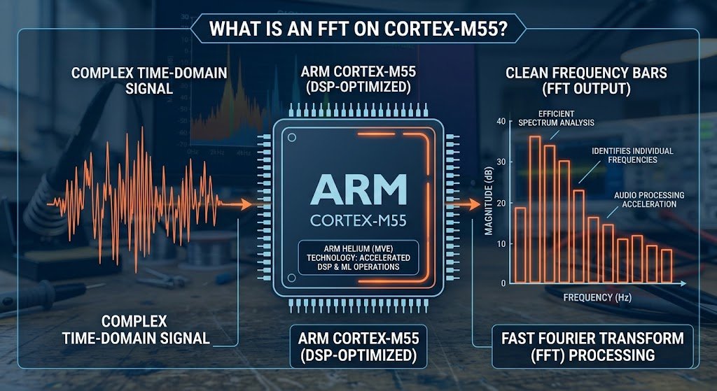
An FFT is an efficient algorithm that converts a signal from the time domain into the frequency domain. In plain terms, it answers the question: which frequencies are present in this signal, and how strong is each one? Think of a piano chord. Your ear hears one sound, but an FFT can separate that sound into the individual notes inside it.
The Cortex-M55 is an Arm processor core designed for embedded devices. It includes Helium, Arm’s vector extension, which processes several data values in a single instruction. That makes it well suited to tasks like audio analysis, vibration monitoring, and filtering.
When you implement an FFT on this core, you usually rely on the CMSIS-DSP library. Arm provides it free of charge, and it contains optimized, tested math functions. You don’t need to write the FFT math yourself. Instead, you feed in your samples and read the results.
Why Does Implementing an FFT on a Cortex-M55 Matter?
Implementing an FFT gives your embedded project several practical advantages:
- Dramatic speed gains: The direct method for a 1024-point transform needs about 1,048,576 complex multiplications, while a radix-2 FFT needs roughly 5,120. This comparison comes from the original 1965 paper by Cooley and Tukey in Mathematics of Computation.
- Vector acceleration: Helium instructions speed up the inner math, so your code finishes sooner.
- Lower power use: Finishing faster lets your chip return to sleep sooner, which saves battery.
- Trusted code: CMSIS-DSP functions are maintained by Arm, so you avoid debugging your own math.
- Real-time response: Your device can analyze live audio or sensor data as it arrives.
Key Facts and Types of FFT on Cortex-M55
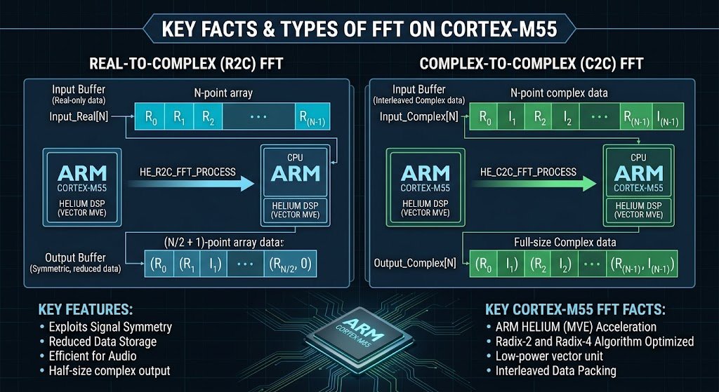
Before you write any code, choose the right FFT type for your data. Arm’s documentation on the CMSIS-DSP library covers each option in detail.
Complex FFT (arm_cfft_f32)
The complex FFT takes samples that include both real and imaginary parts, stored as interleaved pairs. It handles any input, but it needs roughly twice the memory of the real version. Use it when your data is genuinely complex, such as in radio or communications work.
Real FFT (arm_rfft_fast_f32)
Most embedded signals, like microphone or temperature readings, contain only real numbers. The real FFT takes advantage of this symmetry, so it cuts both memory use and processing work. For most projects, this is the best starting point.
Helium (MVE) Acceleration
Helium lets the core handle multiple floating-point or integer values per instruction. CMSIS-DSP uses these instructions when you enable the correct build macros. You get faster code without changing your math.
The table below compares the main options:
| FFT Option | Input Type | Best Use | Memory Needs | Typical Choice |
|---|---|---|---|---|
| Complex FFT (arm_cfft_f32) | Real and imaginary | Radio, communications | Higher | When data is complex |
| Real FFT (arm_rfft_fast_f32) | Real only | Audio, sensors, vibration | Lower | Most embedded projects |
| Direct DFT | Any | Learning, very small sizes | Low | Rarely practical |
How to Implement an FFT on a Cortex-M55
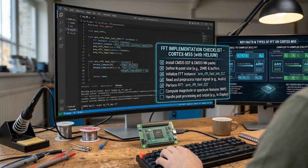
Follow these steps to get your first transform running. If you’re new to the library, read our Chip Support Library: The Easy Guide to CSL for TI DSPs first.
- Install the CMSIS-DSP pack. Add CMSIS-DSP through your IDE’s pack manager, then confirm that your project includes
arm_math.h. Link the library variant that matches your Cortex-M55 target. - Configure the compiler for Cortex-M55 and Helium. Set your target to
-mcpu=cortex-m55and choose the floating-point option your board supports. Define the Helium macro that your CMSIS-DSP version documents so the library uses vector instructions. - Prepare your input buffer. Create a float array whose length matches your FFT size, and fill it with your sampled data. Apply a window, such as Hann, before transforming, because this reduces false peaks at the signal edges.
- Initialize the FFT instance. Call
arm_rfft_fast_init_f32once during startup with your chosen size. Check the returnedarm_statusso you catch unsupported lengths early. - Run the transform. Call
arm_rfft_fast_f32with your input, output buffer, and an inverse flag set to 0 for a forward FFT. The output packs the DC and Nyquist values first, followed by real and imaginary pairs. - Convert the output to frequencies. Use
arm_cmplx_mag_f32to compute each bin’s magnitude, then find the peak. Multiply the peak bin number by your sample rate and divide by the FFT size to get the frequency in hertz.
Here is a minimal example that finds the dominant frequency:
#include "arm_math.h"

#define FFT_SIZE        1024
#define SAMPLE_RATE_HZ  16000

static float32_t fft_input[FFT_SIZE];
static float32_t fft_output[FFT_SIZE];
static float32_t fft_mag[FFT_SIZE / 2];
static arm_rfft_fast_instance_f32 fft_inst;

void fft_init(void) {
    arm_rfft_fast_init_f32(&fft_inst, FFT_SIZE);
}

uint32_t fft_find_peak_hz(void) {
    float32_t max_val;
    uint32_t max_idx;

    arm_rfft_fast_f32(&fft_inst, fft_input, fft_output, 0);
    arm_cmplx_mag_f32(&fft_output[2], fft_mag, FFT_SIZE / 2 - 1);
    arm_max_f32(fft_mag, FFT_SIZE / 2 - 1, &max_val, &max_idx);

    return (max_idx + 1) * SAMPLE_RATE_HZ / FFT_SIZE;
}
Common Mistakes and Myths to Avoid
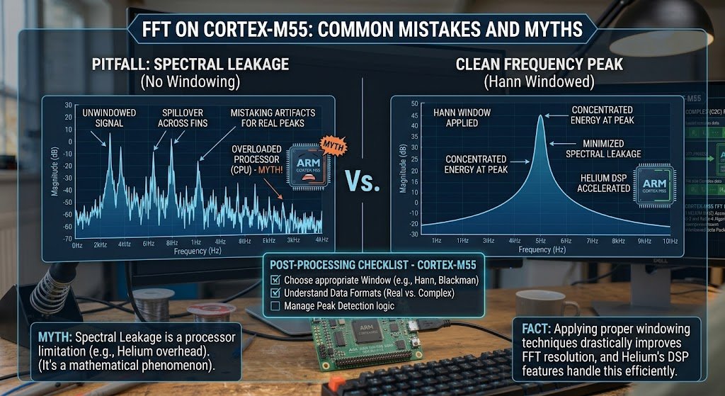
Myth: A bigger FFT is always better. Larger sizes give finer frequency resolution, but they use more memory and take longer to compute. Choose the smallest size that resolves the frequencies you care about.
Mistake: Ignoring the sample rate. Each bin’s frequency depends on your sample rate. If that value is wrong, every frequency you report will also be wrong.
Myth: Helium turns on automatically. The vector speedup requires the correct compiler flags and macros. Without them, your results stay correct, but the code runs more slowly.
Mistake: Skipping windowing. Without a window, abrupt signal edges create false peaks called spectral leakage. Apply a Hann window to most general-purpose signals.
Mistake: Using the complex FFT for real data. This doubles memory use and processing work with no benefit. Use the real FFT for sensor and audio data.
Expert Tips for Best Results
- Precompute your window coefficients once at startup, not inside your processing loop.
- Use DMA to fill the input buffer, so the CPU can spend its time on processing.
- Keep FFT buffers in fast on-chip RAM and follow your toolchain’s alignment guidance.
- Measure timing with the DWT cycle counter to see the real performance on your board.
- Test with a known sine wave first, such as a 1 kHz tone, to confirm the peak lands in the correct bin.
Frequently Asked Questions
Do I need to write my own FFT code on Cortex-M55?
No. The CMSIS-DSP library provides optimized, tested FFT functions for Cortex-M55, so you can call them directly. Writing your own FFT is a useful learning exercise, but production projects almost always benefit from Arm’s maintained code and Helium acceleration. Start with the library, then study its source code if you want to understand what happens inside.
What FFT size should I choose for my project?
Pick a size that gives you enough frequency resolution for your signal. Frequency resolution equals your sample rate divided by the FFT size, so a 1024-point FFT sampling at 16 kHz gives about 15.6 Hz per bin. Choose a power of two that balances accuracy against memory and processing time.
Is an FFT on Cortex-M55 fast enough for real-time audio?
Often, yes, especially with Helium and the real FFT. Real-time means finishing each block before the next one arrives, so compare your measured cycle count against your block period. If your code runs too slowly, reduce the FFT size or sample rate, and confirm the timing with the DWT cycle counter.
Final Thoughts
Implementing an FFT on a Cortex-M55 is more approachable than most people expect. Three ideas matter most. First, an FFT converts a time signal into its frequency content far faster than the direct method. Second, the real FFT in CMSIS-DSP is the best starting point for sensor and audio data. Third, correct sample rate handling and windowing decide whether your results are trustworthy.
Start today: install CMSIS-DSP, feed a 1 kHz test tone through your first transform, and check that the peak lands where it should. Then build from there.
What signal would you like your Cortex-M55 to analyze first? Share your project idea in the comments below.