
The sampling theorem (the Nyquist–Shannon theorem) says that a signal containing no frequencies above fmax can be rebuilt perfectly from its samples, provided the sample rate fs is more than twice fmax. That minimum rate, 2 × fmax, is called the Nyquist rate, sample slower than it, and the signal’s high frequencies fold back as false low frequencies: aliasing.
What the sampling theorem says, in plain English
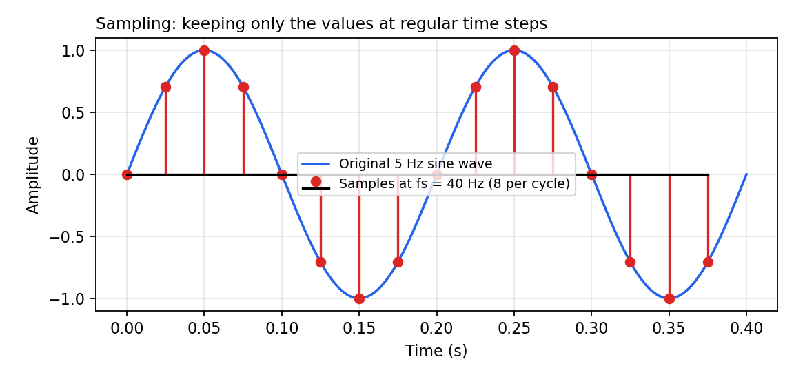
Sampling turns a continuous signal, a voltage, a sound wave, into a list of numbers, keeping only the value at evenly spaced moments. The obvious worry: everything between those moments is thrown away, so how could the original ever be recovered? The sampling theorem answers that worry with a guarantee. If the signal is bandlimited (it contains no frequency higher than some fmax) and you sample faster than twice that highest frequency, then nothing is lost. The original waveform is the only bandlimited signal that passes through your samples, so in principle it can be reconstructed exactly.
The theorem is the foundation under every ADC, every audio interface and every digital recording. Our lesson on what a signal is in DSP covers the continuous-to-digital step itself; this lesson covers the rule that makes that step safe.
Why twice the highest frequency?
Think of the fastest wiggle in the signal. To capture a wiggle you need, at minimum, a sample near its peak and a sample near its trough, two samples per cycle. Sample less often than that and a fast wiggle can hide between your samples, or worse, masquerade as a slower wiggle. That is the whole intuition: at least two samples per cycle of the highest frequency present. Formally:
fs > 2 × fmax (the sampling condition)
Two terms students constantly swap, keep them separate:
| Term | Meaning | Example (fmax = 3 kHz) |
|---|---|---|
| Nyquist rate | The minimum sample rate for this signal: 2 × fmax. A property of the signal. | 6 kHz |
| Nyquist frequency | Half of the sample rate you actually chose: fs / 2. A property of the sampler. Frequencies above it fold back. | At fs = 10 kHz, the Nyquist frequency is 5 kHz |
The rule, restated with the second term: your signal’s fmax must sit below the Nyquist frequency.
Worked example: a signal with 1 kHz and 3 kHz parts
A sensor signal contains a 1 kHz tone and a weaker 3 kHz tone, and nothing higher. Then fmax = 3 kHz, so:
- Nyquist rate = 2 × 3 kHz = 6 kHz. Sampling must be strictly faster than this.
- Sampling at exactly 6 kHz is a knife-edge, it only works for a perfectly behaved signal, so engineers leave margin.
- Sampling at 10 kHz gives a Nyquist frequency of 5 kHz: both tones (1 and 3 kHz) sit safely below it, and a real anti-aliasing filter has room to work.
- Sampling at 5 kHz breaks the rule: the 3 kHz tone is above the 2.5 kHz Nyquist frequency and folds to |3 − 5| = 2 kHz, a false tone that no later processing can remove.
That folding calculation, and how to prevent it, is the whole subject of our aliasing lesson, read it next if the last bullet is the part you need most.
Reconstruction: how the samples become a signal again
The theorem is not just a promise, it comes with the recipe. Each sample is replaced by a sinc pulse, scaled by the sample value, and all the pulses are added. Where the pulses overlap they reinforce and cancel in exactly the way needed to rebuild the original curve:
x(t) = Σn x[n] · sinc((t − nT) / T), where T = 1 / fs
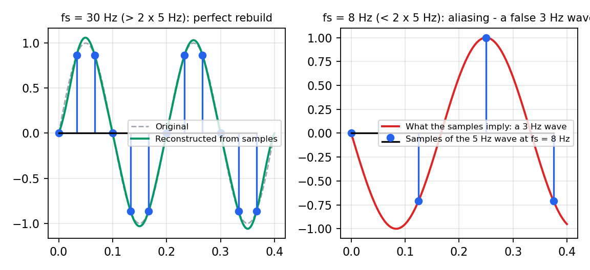
In practice DACs approximate this with simpler filters, but the sinc sum is what they approximate. Below, a 5 Hz tone sampled at 30 Hz is rebuilt this way and lands back on the original; the same tone sampled at 8 Hz cannot be rebuilt at all, its samples sit exactly on a different, 3 Hz wave:
Sampling theorem in Python (tested code)
This code samples a 5 Hz tone two ways and checks the alias claim numerically, the samples taken at 8 Hz match a 3 Hz wave at every sample point:
import numpy as np

f = 5.0                      # tone frequency, Hz

# Fast enough: fs = 30 Hz > 2 * 5 Hz
fs_good = 30.0
t_good = np.arange(0, 1.0, 1 / fs_good)
x_good = np.sin(2 * np.pi * f * t_good)   # samples that keep the signal

# Too slow: fs = 8 Hz < 2 * 5 Hz -> aliasing
fs_low = 8.0
t_low = np.arange(0, 2.0, 1 / fs_low)
x_low = np.sin(2 * np.pi * f * t_low)

alias = -np.sin(2 * np.pi * 3.0 * t_low)  # a 3 Hz wave, sign flipped
print(np.allclose(x_low, alias))          # True: the samples cannot
                                          # tell 5 Hz from 3 Hz
The alias frequency follows the folding rule from the aliasing lesson: |f − k·fs| = |5 − 8| = 3 Hz. Once two different signals produce identical samples, no algorithm can know which one was real, that information is gone, which is why the sampling condition is a hard rule and not a guideline.
Sample rates you already know, checked against the theorem
| System | Sample rate | Highest frequency it must capture | Nyquist check |
|---|---|---|---|
| CD audio | 44.1 kHz | ~20 kHz (limit of hearing) | Nyquist frequency 22.05 kHz > 20 kHz ✓ |
| Studio / video audio | 48 kHz | ~20 kHz | 24 kHz > 20 kHz ✓, with more filter margin |
| Telephone voice | 8 kHz | ~3.4 kHz (voice band) | 4 kHz > 3.4 kHz ✓, enough for speech, not music |
| High-resolution audio | 96–192 kHz | ~20 kHz | Far above the minimum; the extra room eases filter design |
Notice the pattern: real systems always sample somewhat above the bare Nyquist rate. The margin is not waste, a real anti-aliasing filter cannot cut off infinitely sharply at fmax, so the gap between fmax and the Nyquist frequency is where that filter does its work.
Common mistakes
- Swapping Nyquist rate and Nyquist frequency. The rate (2 × fmax) belongs to the signal; the frequency (fs / 2) belongs to the sampler. Mixing them up inverts the design rule.
- Sampling at exactly 2 × fmax. The theorem needs more than twice. At exactly twice, a sine at fmax can be sampled at its zero crossings and vanish entirely.
- Assuming the theorem fixes a bad recording. It is a guarantee about information, not a repair tool: if aliasing happened at capture, it is permanent.
- Forgetting the bandlimited condition. Real signals are never perfectly bandlimited, which is why the anti-aliasing filter before the ADC matters as much as the sample rate.
Quick quiz
- A signal contains frequencies up to 7 kHz. What is its Nyquist rate?
- You sample at 16 kHz. What is the Nyquist frequency, and can the system capture a 9 kHz tone faithfully?
- Why do real systems sample above the Nyquist rate instead of exactly at it?
Answers
- 14 kHz, and in practice you would sample strictly above it.
- The Nyquist frequency is 8 kHz. No: 9 kHz is above it and would fold to |9 − 16| = 7 kHz.
- Because anti-aliasing filters need a transition band between fmax and the Nyquist frequency, and exactly 2 × fmax fails for worst-case signals.
Frequently asked questions
What is the sampling theorem in simple words?
The sampling theorem says a smooth, bandlimited signal can be captured perfectly by measuring it at regular intervals, as long as you measure more than twice as fast as its highest frequency wiggles. Sample slower than that and fast wiggles disguise themselves as slow ones, aliasing, and the original can no longer be recovered.
What happens if you sample below the Nyquist rate?
Frequencies above half the sample rate fold back into the measured band as false, lower frequencies. A 3 kHz tone sampled at 5 kHz appears at 2 kHz, mixed permanently with any real 2 kHz content. Because different original signals produce identical samples, no later filtering or software can undo the damage.
Why is CD sample rate 44.1 kHz?
Human hearing tops out near 20 kHz, so the sampling theorem demands a rate above 40 kHz. The CD standard chose 44.1 kHz: high enough to place the Nyquist frequency at 22.05 kHz, leaving a 2.05 kHz transition band for the anti-aliasing filter, while keeping the data rate as low as 1980s hardware allowed.
Does a higher sample rate always mean better quality?
No. Once the sample rate comfortably exceeds twice the highest frequency present, the theorem says the bandlimited signal is already captured completely. Higher rates can make filter design easier and are useful in production, but they add no new information about a signal that was already sampled correctly.
Where to go next
The sampling theorem tells you how fast to sample; convolution tells you what a system does to the samples afterwards. If you have not seen it yet, the aliasing lesson is this theorem’s warning label, with its own worked Python example. The full order is on the Beginner DSP learning path.
References
- Steven W. Smith, The Scientist and Engineer’s Guide to Digital Signal Processing, Chapter 3, “ADC and DAC”, dspguide.com/ch3.htm
- “Nyquist–Shannon sampling theorem”, Wikipedia, en.wikipedia.org/wiki/Nyquist–Shannon_sampling_theorem
Try it yourself
Do not take the folding on faith, cause it. Pick a tone in the demo, lower the sample rate step by step, and watch the alias appear at exactly |f − fs| when you cross the Nyquist limit. Open the Aliasing and Nyquist Demo. For rate conversions and dB math while you design, the dB and Sample-Rate Calculators sit on the same tools page family.
Keep going in order: the Beginner DSP learning path shows what to learn next.