
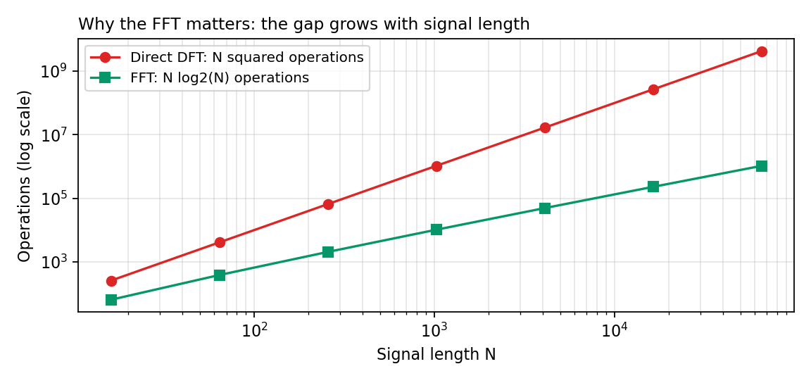
The DFT and the FFT are not two different transforms. The DFT (Discrete Fourier Transform) is the mathematical operation that converts N time samples into N frequency values. The FFT (Fast Fourier Transform) is a family of clever algorithms that compute exactly the same DFT, identical results, no approximation, using roughly N·log₂N operations instead of N², which at a million samples is about 50,000 times less work.
What is the DFT?
The DFT answers one question about a finite signal: how much of each frequency does it contain? Give it N samples x[0]…x[N−1] and it returns N frequency values X[0]…X[N−1], one for each frequency the signal can represent, from 0 Hz up to just under the sample rate. Each value is complex, it carries both the strength of that frequency and its phase.
The definition is a single sum, applied once per output frequency k:
X[k] = Σn=0N−1 x[n] · e−j2πkn/N
Read it as a matching test: for frequency k, multiply the signal by a complex wave of that frequency and add everything up. If the signal really contains that frequency, the products line up and the sum is large; if not, they cancel and the sum is near zero. The DFT is the frequency-domain view of the same signal, the partner of the time-domain view in our signals lesson, and the discrete cousin of the Fourier series.
What is the FFT?
The FFT is not a transform at all, it is a recipe for computing the DFT quickly. The direct sum above repeats almost identical multiplications millions of times. FFT algorithms (the classic one is Cooley–Tukey, 1965) notice that a DFT of length N can be split into two DFTs of length N/2, one over the even samples, one over the odd samples, whose results combine cheaply. Split again and again, and the repeated work collapses. That splitting is exactly the decimation-in-time idea in our DIT FFT lesson, which walks through the butterfly diagrams step by step.
The crucial point, and the one most often gotten wrong: the FFT output is the DFT output, digit for digit (up to floating-point rounding). “FFT” names the shortcut, “DFT” names the destination.
DFT vs FFT, side by side
| DFT | FFT | |
|---|---|---|
| What it is | A mathematical transform: N samples → N frequency values | An algorithm family that computes the DFT |
| Result | X[k], the spectrum | The same X[k], identical values |
| Cost | ~N² operations | ~N·log₂N operations |
| N = 1,024 | ~1,048,576 operations | ~10,240 operations (≈100× less) |
| N = 1,000,000 | ~10¹² operations | ~2 × 10⁷ operations (≈50,000× less) |
| When you say it | Discussing theory, formulas, properties | Discussing the computation or the library call |
Worked example: the DFT of [1, 2, 3, 4]
Take x = [1, 2, 3, 4], so N = 4. The DFT has four outputs. X[0] is always just the sum of the samples: 1 + 2 + 3 + 4 = 10 (the “DC” or average component). X[1] uses the matching-test sum with k = 1:
X[1] = 1·(1) + 2·(−j) + 3·(−1) + 4·(j) = −2 + 2j
The four complex exponentials for N = 4 simply cycle through 1, −j, −1, j. Completing the same calculation for k = 2 and k = 3 gives the full result:
X = [10, −2 + 2j, −2, −2 − 2j]
Notice X[1] and X[3] are mirror images (complex conjugates), that symmetry always appears for real-valued input signals, and it is why tools usually only plot the first half of the spectrum. Every number here is reproduced exactly by the Python code below.
What a spectrum looks like
For a real signal, two sine tones at 50 Hz and 120 Hz, sampled at 1,000 Hz, the DFT magnitude has one peak per tone, at the right frequency and the right height:
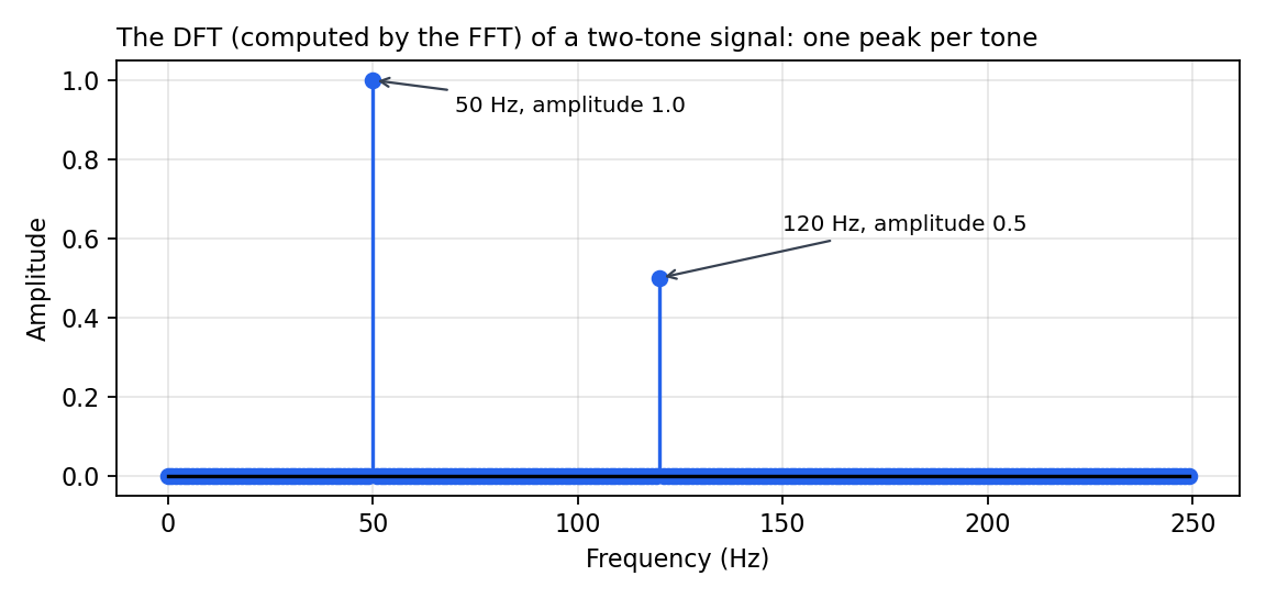
You can produce this exact plot in your browser, no code, with our FFT Visualizer, change the tones and watch the peaks move.
DFT and FFT in Python (tested code)
Here is the definition written out as a loop, checked against NumPy’s FFT on the worked example. Both return identical values:
import numpy as np

def dft_manual(x):
    N = len(x)
    X = np.zeros(N, dtype=complex)
    for k in range(N):                       # each output frequency
        for n in range(N):                   # the matching-test sum
            X[k] += x[n] * np.exp(-2j * np.pi * k * n / N)
    return X

x = np.array([1.0, 2.0, 3.0, 4.0])
print(dft_manual(x))        # [10.+0.j -2.+2.j -2.+0.j -2.-2.j]
print(np.fft.fft(x))        # [10.+0.j -2.+2.j -2.+0.j -2.-2.j]
print(np.allclose(dft_manual(x), np.fft.fft(x)))   # True
The loop is the DFT definition and nothing else, which is precisely why it is slow. np.fft.fft runs an FFT algorithm under the hood, so for real work you always call the library; the manual version exists so the formula is never a black box. This speed difference is also why fast convolution works: convolving via two FFTs, a multiply, and an inverse FFT beats the direct method on long signals. And when a signal changes over time, the STFT simply runs this same FFT on window after window.
When does the difference actually matter?
- Short signals: for a few dozen samples, the direct DFT is fine and sometimes clearer. The FFT’s advantage is real but small.
- Real-time audio: a 48 kHz stream processed in blocks of 4,096 samples needs an FFT millions of times a day, the N² version would not keep up; the FFT does it easily, including on small embedded chips (see our FFT on a Cortex-M55 lesson).
- Long recordings and images: at N in the millions, the direct DFT is not “slower”, it is simply not an option.
- Exam questions: if a question asks you to “compute the DFT”, it wants the sum and the values. If it asks about the FFT, it wants the splitting trick and the N·log₂N cost.
Common mistakes
- “The FFT is an approximation of the DFT.” It is not. Same inputs, same outputs, only the arithmetic is reorganised.
- “Zero-padding improves frequency resolution.” Padding a signal with zeros before the FFT interpolates the spectrum, the plot gets smoother, but two close tones that merged before still merge. True resolution comes from a longer recording.
- Reading all N outputs as N different frequencies. For real signals the second half mirrors the first; the unique content lives in the first N/2 + 1 values (which is what
np.fft.rfftreturns). - Forgetting the sample rate. The DFT gives bin numbers k, not Hertz. The frequency of bin k is k × fs / N, without fs the spectrum has no physical scale.
Quick quiz
- True or false: an FFT of a signal gives slightly different values than its DFT.
- Roughly how many operations does an FFT of 1,024 samples need, versus a direct DFT?
- Your DFT output has a peak at bin k = 10, with N = 500 and fs = 1,000 Hz. What frequency is the peak?
Answers
- False, the FFT computes the DFT exactly (up to floating-point rounding).
- About 10,240 operations (N·log₂N) versus about 1,048,576 (N²), roughly 100× less.
- k × fs / N = 10 × 1000 / 500 = 20 Hz.
Frequently asked questions
Is the FFT the same as the DFT?
The FFT is an algorithm; the DFT is the transform it computes. Asking whether they are the same is like asking whether long division is the same as division: one is the procedure, the other is the operation. FFT results equal DFT results for the same input, the difference is speed, never the answer.
Why is the FFT so much faster than the direct DFT?
The direct DFT recomputes nearly identical products for every output frequency, costing about N² operations. The FFT splits the DFT into two half-size DFTs over the even and odd samples, reuses their results, and splits recursively, costing about N·log₂N operations. At a million samples that is roughly 50,000 times less arithmetic.
What is the difference between the DFT and the FFT in an exam?
Examiners use “DFT” when they want the transform itself: the summation formula, a hand-computed spectrum, or properties such as symmetry for real signals. They use “FFT” when they want the computation: the radix-2 splitting, butterfly diagrams, or the N·log₂N complexity. Knowing which word was used tells you which half of this lesson to answer from.
Does the FFT work for any signal length?
The classic radix-2 FFT is fastest when N is a power of two, which is why tools often pad signals to 256, 1,024 or 4,096 samples. Modern libraries such as NumPy and FFTW handle other lengths efficiently too, by mixing smaller factorizations, the DFT result is still exact, just computed with a less regular splitting pattern.
Where to go next
Now that the DFT/FFT distinction is settled, the natural next steps are how the FFT’s splitting works in detail (Decimation-in-Time) and how the transform behaves on a real microcontroller (FFT on Cortex-M55). The full order is on the Beginner DSP learning path.
References
- Steven W. Smith, The Scientist and Engineer’s Guide to Digital Signal Processing, Chapter 8, “The Discrete Fourier Transform”, dspguide.com/ch8.htm
- NumPy documentation: numpy.fft.fft
- SciPy documentation: scipy.fft.fft
Try it yourself
Build a signal from two tones and read its DFT in the browser, then change one tone and predict where the peak moves before you look. Open the FFT Visualizer.
Keep going in order: the Beginner DSP learning path shows what to learn next.